This post is directed primarily at physics students and instructors and stems from discussions with my colleague Prof. Matt Moelter at Cal Poly, SLO. In introductory electrostatics there is a standard result involving the electric field near conducting and non-conducting surfaces that confuses many students.
Near a non-conducting sheet of charge with charge density  , a straightforward application of gauss’s law gives the result

While, near the surface of a conductor with charge density , again, an application of gauss’s law gives the result

The latter result comes about because the electric field inside a conductor in electrostatic equilibrium is zero, killing off the flux contribution of the gaussian pillbox inside the conductor. In the case of the sheet of charge, this same side of the pillbox distinctly contributed to the flux. Both methods are applied locally to small patches of their respective systems.
Although the two equations are derived from the same methods, they mean different things — and their superficial resemblance within factors of two can cause conceptual problems.
In Equation (1) the relationship between and  is causal. That is, the electric field is due directly from the source charge density in question. It does not represent the field due to all sources in the problem, only the lone contribution from that local .
In Equation (2) the relationship between and is not a simple causal one, rather it expresses self-consistentancy, discussed more below. Here the electric field represents the net field outside of the conductor near the charge density in question. In other words, it automatically includes both the contribution from the local patch itself and the contributions from all other sources. It is has already added up all the contributions from all other sources in the space around it (this could, in some cases, include sources you weren’t aware of!).
How did this happen? First, in contrast to the sheet of charge where the charges are fixed in space, the charges in a conductor are mobile. They aren’t allowed to move while doing the “statics” part of electrostatics, but they are allowed to move in some transient sense to quickly facilitate a steady state. In steady state, the charges have all moved to the surfaces and we can speak of an electrostatic surface distribution on the conductor. This charge mobility always arranges the surface distributions to ensure  inside the conductor in electrostatic equilibrium. This is easy enough to implement mathematically, but gives rise to the subtle state of affairs encountered above. The on the conductor is responding to the electric fields generated by the presence of other charges in the system, but those other charges in the system are, in turn, responding to the local in question. Equation (2) then represents a statement of self-consistency, and it breaks the cycle using the power of gauss’s law. As a side note, the electric displacement vector,
  , plays a similar role of breaking the endless self-consistency cycle of polarization and electric fields in symmetric dielectric systems.
Let’s look at some examples.
Example 1:
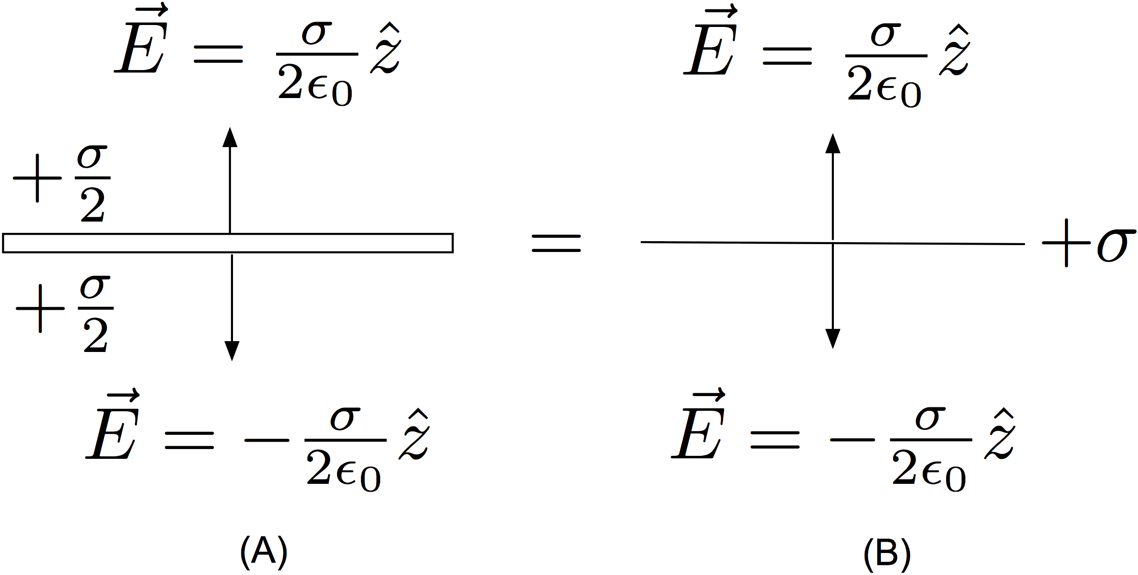
Consider a large conducting plate versus large non-conducting sheet of charge. Each surface is of area A. The conductor has total charge Q, as does the non-conducting sheet. Find the electric field of each system. The result will be that the fields are the same for the conductor and non-conductor, but how can this be reconciled with Equation (1) and (2) which, at a glance, seem to give very different answers? See the figure below:
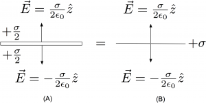
For the non-conducting sheet, as shown in Figure (B) above, the electric field due to the source charge is given by Equation (1)

where

(“nc” for non-conducting) and  above the positive surface and
  below it.
Now, in the case of the conductor, shown in Figure (A), Equation (2) tells us the net value of the field outside the conductor. This net value is expressed, remarkably, only in terms of the local charge density; but remember, for a conductor, the local charge density contains information about the entire set of sources in the space. At a glance, it seems the electric field might be twice the value of the non-conducting sheet. But no! This is because the charge density will be different than the non-conducting case. For the conductor, the charge responds to the presence of the other charges and spreads out uniformly over both the top and bottom surface; this ensures inside the conductor. In this context, it is worth point out that there are no infinitely thin conductors. Infinitely thin sheets of charge are fine, but not conductors. There are always two faces to a thin conducting surface and the surface charge density must be (at least tacitly) specified on each. Even if a problem uses language that implies the conducting surface is infinitely thin, it can’t be.
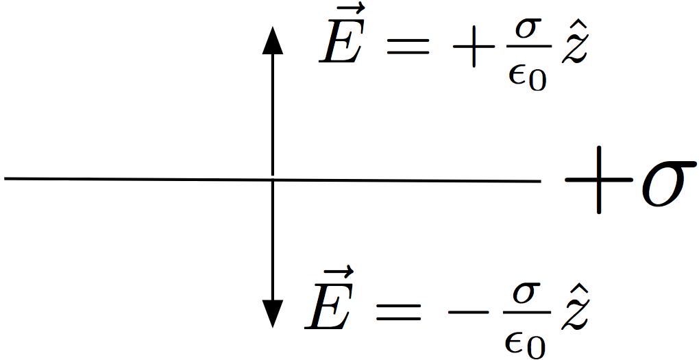
For example, the following Figure for an “infinitely thin conducting surface with charge density “, which then applies Equation (2) to the setup to determine the field, makes no sense:
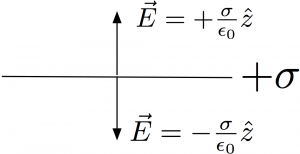
This application of Equation (2) cannot be reconciled with Equation (1). We can’t have it both ways. An “infinitely thin conductor” isn’t a conductor at all and should reduce to Equation (1). To be a conductor, even a thin one, there needs to be (at least implicitly) two surfaces and a material medium we call “the conductor” that is independent of the charge.
Back to the example.
If the charge Q is spread out uniformly over both sides of the conductor in Figure (A), the charge density for the conductor is then

(“c” for conducting). The factor of 2 comes in because each face has area A and the charge spreads evenly across both. Equation (2) now tells us what the field outside the conductor is. This isn’t just for the one face, but includes the net contributions from all sources
 .
.
That is, the net field is the same for each case,
 .
.
Even though Equations (1) and (2) might seem superficially inconsistent with each other for this situation, they give the same answer, although for different reasons. Equation (1) gives the electric field that results directly from alone. Equation (2) gives a self consistent net field outside the conductor, which uses information contained in the local charge density. The key is understanding that the surface charge density used for the sheet of charge and the conductor are different in each case. In the case of a charged sheet, we have the freedom to declare a surface with a fixed, unchanging charge density. With a conductor, we have less, if any, control over what the charges do once we place them on the surfaces.
It is worth noting that each individual surface of charge on the conductor has a causal contribution to the field still given by Equation (1), but only once the surface densities have been determined — with one important footnote. The net field in each region can be determined by adding up all the (shown) individual contributions in superposition only if the charges shown are the only charges in the problem and were allowed to relax into this equilibrium state due to the charges explicitly shown. This last point will be illustrated in an example at the end of this post. It turns out that you can’t just declare arbitrary charge distributions on conductors and expect those same charges you placed to be solely responsible for it. There may be “hidden sources” if you insist on keeping your favorite arbitrary distribution on a conductor. If you do, you must also account for those contributions if you want to determine the net field by superposition. However, all is not lost: amazingly, Equation (2) still accounts for those hidden sources for the net field! With Equation (2) you don’t need to know the individual fields from all sources in order to determine the net field. The local charge density on the conductor already includes this information!
Example 2:
Compare the field between a parallel plate capacitor with thin conducting sheets each having charge  and area A with the field between two non-conducting sheets of charge with charge and area A. This situation is a standard textbook problem and forms the template for virtually all introductory capacitor systems. The result is that the field between the conducting plates are the same as the field between the non-conducting charge sheets, as shown in the figure below. But how can this be reconciled with Equations (1) and (2)? We use a treatment similar to those in Example 1.
Between the two non-conducting sheets, as shown in Figure (D), the top positive sheet has a field given by Equation (1), pointing down (call this the  direction) . The bottom negative sheet also has a field given by Equation (1) and it also points down. The charge density on the positive surface is given by
  . We superimpose the two fields to get the net result
 .
.
Above the top positive non-conducting sheet the field points up due to the top non-conducting sheet and down from the negative non-conducting sheet. Using Equation (1) they have equal magnitude, thus the fields cancel in this region after superposition. The fields cancel in a similar fasshion below the bottom non-conducting sheet.
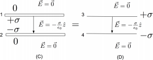
Unfortunately, the setup for the conductor, shown in Figure (C), is framed in an apparently ambiguous way. However, this kind of language is typical in textbooks. Where is this charge residing exactly? If this is not interpreted carefully, it can lead to inconsistencies like those of the “infinite thin conductor” above. The first thing to appreciate is that, unlike the nailed down charge on the non-conducting sheets, the charge densities on the parallel conducting plates are necessarily the result of responding to each other. The term “capacitor” also implies that we start with neutral conductors and do work bringing charge from one, leaving the other with an equal but opposite charge deficit. Next, we recognize even thin conducting sheets have two sides. That is, the top sheet has a top and bottom and the bottom conducting sheet also has a top and bottom. If the conducting plates have equal and opposite charges, and those charges are responding to each other. They will be attracted to each other and thus reside on the faces that are pointed at each other. The outer faces will contain no charge at all. That is, the from the top plate is on that plate’s bottom surface with none on the top surface. Notice, unlike Example 1, the conductor has the same charge density as its non-conducting counterpart. Similar for the bottom plate but with the signs reversed. A quick application of gauss’s law can also demonstrate the same conclusion.
With this in mind, we are left with a little puzzle. Since we know the charge densities, do we jump right to the answer using Equation (2)? Or do we now worry about the individual contributions of each plate using Equation (1) and superimpose them to get the net field? The choice is yours. The easiest path is to just use Equation (2) and write down the results in each region. Above and below all the plates,  so $\vec{E}=0$; again, Equation (2) has already done the superposition of the individual plates for us. In the middle, we can use either plate (but not both added…remember, this isn’t superposition!). If we used the top plate, we would get

and if we used the bottom plate alone, we would get
 .
.
They both give the same individual result, which is the same result as the non-conducting sheet case above where we added individual contributions.
If were were asked “what is the force of the top plate on the bottom plate?” we actually do need to know the field due to the charge on the single top plate alone and apply it to the charge on the second plate. In this case, we are not just interested in the total field due to all charges in the space as given by Equation (2). In this case, the field due to the single top plate would indeed be given by Equation (1), as would the field due to the single bottom plate. We could then go on to superimpose those fields in each region to obtain the same result. That is, once the charge distributions are established, we can substitute the sheets of non-conducting charge in place of the conducting plates and use those field configurations in future calculations of energy, force, etc.
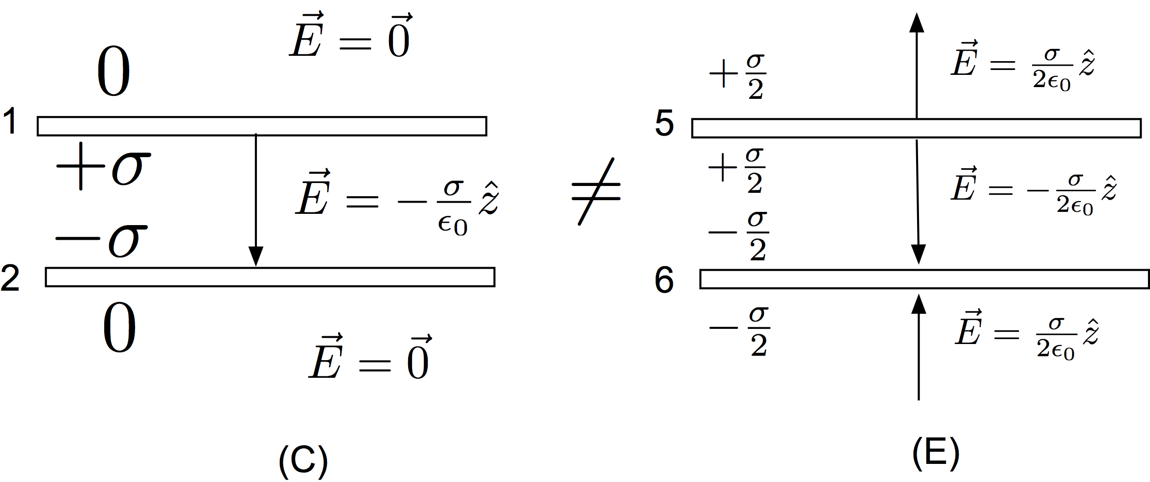
However, not all charge distributions for the conductor are the same. A strange consequence of all this is that, despite the fact that Example 1 gave us one kind of conductor configuration that was equivalent to single non-conducting sheet, this same conductor can’t be just transported in and made into a capacitor as shown in the next figure:

On a conductor, we simply don’t have the freedom to invent a charge distribution, declare “this is a parallel plate capacitor,” and then assume the charges are consistent with that assertion. A charge configuration like Figure (E) isn’t a parallel plate capacitor in the usual parlance, although the capacitance of such a system could certainly be calculated. If we were to apply Equation (1) to each surface and superimpose them in each region, we might come to the conclusion that it had the same field as a parallel plate capacitor and conclude that Figure (E) was incorrect, particularly in the regions above and below the plates. However, Equation (2) tells us that the field in the region above the plates and below them cannot be zero despite what a quick application of Equation (1) might make us believe. What this tells us is that there must unseen sources in the space, off stage, that are facilitating the ongoing maintenance of this configuration. In other words, charges on conducting plates would not configure themselves in such a away unless there were other influences than the charges shown. If we just invent a charge distribution and impose it onto a conductor, we must be prepared to justify it via other sources, applied potentials, external fields, and so on.
So, even though plate (5) in Figure (E) was shown to be the same as a single non-conducting plate, we can’t just make substitutions like those in this figure. We can do this with sheets of charge, but not with other conductors. Yes, the configuration in Figure (E) is physically possible, it just isn’t the same as a parallel plate capacitor, even though each element analyzed in isolation makes it seem like it would be the same.
In short, Equations (1) and (2) are very different kinds of expressions. Equation (1) is a causal one that can be used in conjunction with the superposition principle: one is calculating a single electric field due to some source charge density. Equation (2) is more subtle and is a statement of self-consistency with the assumptions of a conductor in equilibrium. An application of Equation (2) for a conductor gives the net field due to all sources, not just the field do to the conducting patch with charge density sigma: it comes “pre-superimposed” for you.

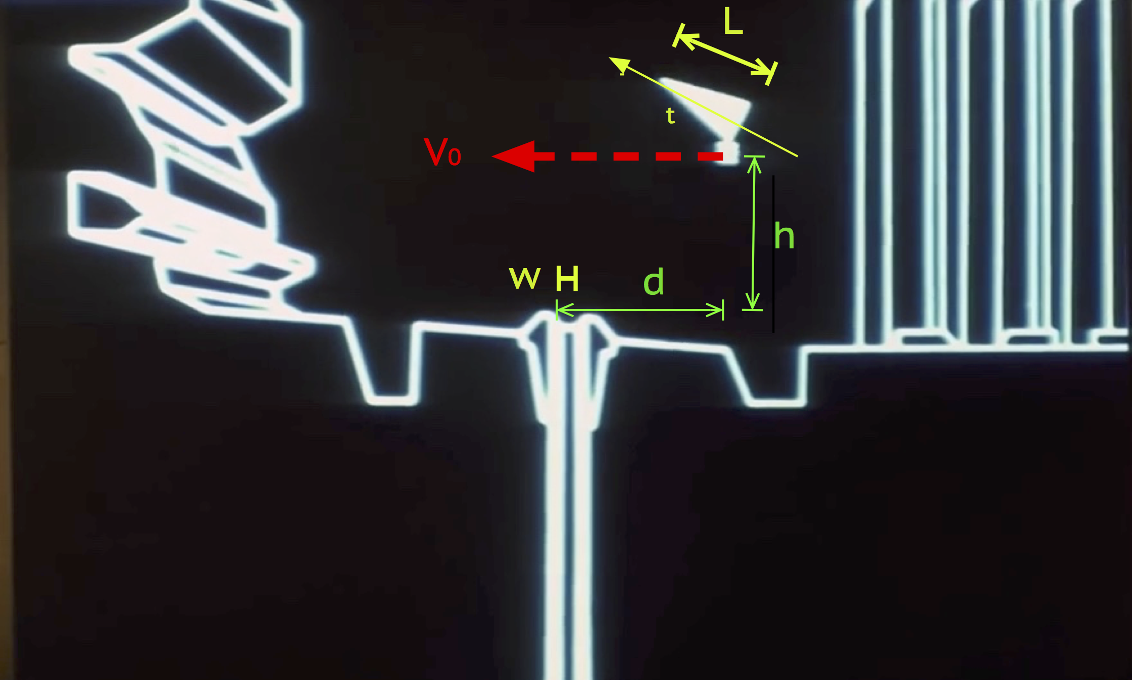

 = 0 degrees and h = d, the formula simplifies to
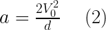 .
. .
.
 is the useful energy extracted from a mass
  with efficiency
  . The mass is converted to a volume using the density of the material.
 required to accelerate an object of mass M to a light-speed fraction
  at efficiency
  .
.


 clearly we recover N1, which can now be stated something like: