This is the second in a two part post where I calculate the size and mass respectively of the Death Star in Episode IV (DS1). Estimating the mass will inform discussion about the power source of the station and other energy considerations.
Part II: Mass of DS1
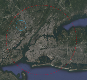
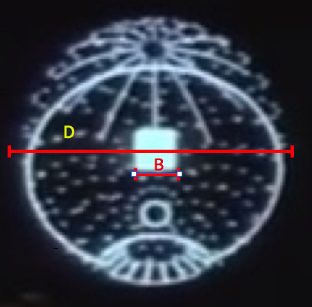
As argued in Part I, I assert that the diameter of DS1 is approximately 60 km based on a self-consistent scale analysis of the station plan schematics as shown during the briefing prior to the Battle of Yavin.
A “realistic” upper limit for the mass is set if the 60 km volume of DS1 was filled with the densest (real, stable) element currently known. This is osmium with a mass density of 2.2E4 kilograms per cubic meter. This places the mass at 2.5E18 kg with a surface gravity of 0.05g. A filling fraction of 10% would then place a “realistic” estimate of the upper limit at 2.5E17 kg. Other analyses have made similar assessments using futuristic materials with some volume filling-fraction, also putting the mass somewhere around 10^18 kg assuming a radius of 160 km.
In this mass analysis, using information from the available footage from the Battle of Yavin, I find a DS1 mass of roughly 2.8E23 kg, about million times the mass of a “realistic” approximation Any supporting superstructure would be a small perturbation on this number. This implies a surface gravity of an astounding 448g. To account for this, my conclusion is that DS1 has a 40 m radius sphere of (contained) quark-gluon plasma or a 55 m radius quantity of neutronium at its core. Such materials, if converted to useful energy with an efficiency of 0.1%, would be ample to 1) provide the 2.21E32 J/shot of energy required to destroy a planet as well as 2) serve as a power source for sub-light propulsion.
Details
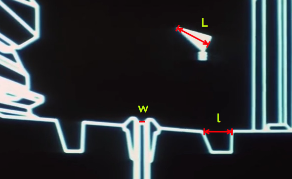
The approach here uses the information available in the schematics shown during the briefing. The briefing displays a simulation of the battle along the trench to the exhaust port. Again, as shown in Part I of this post, the simulation scale is self-consistent with other scales in both the schematic and the actual battle footage. As shown in Figure 1, the proton torpedo is launched into projectile motion only under the influence of gravity. It appears to be at rest with respect to the x-wing as it climbs at an angle of about 25 degrees.
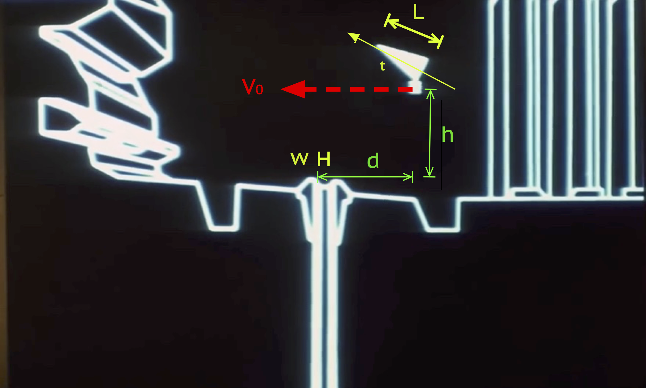
Figure 1
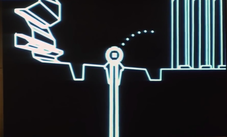
Figure 2
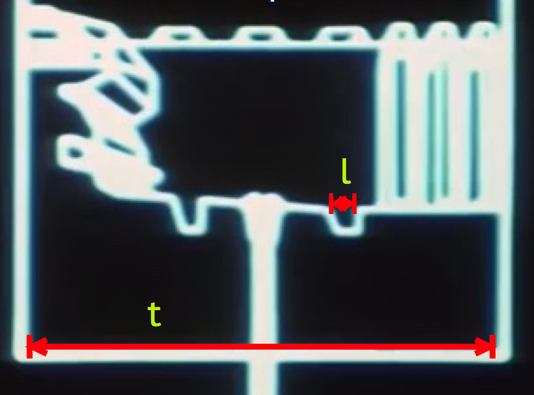
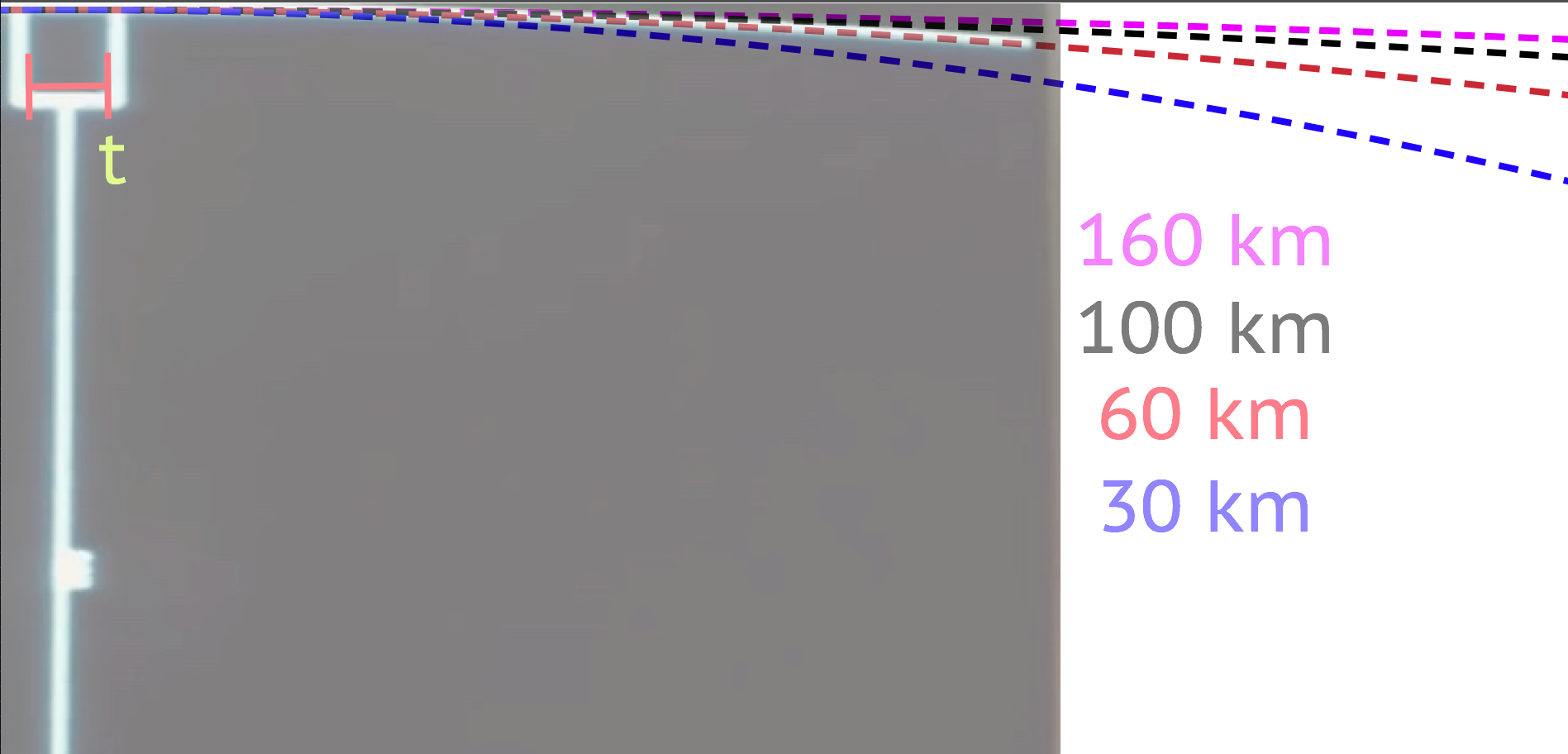
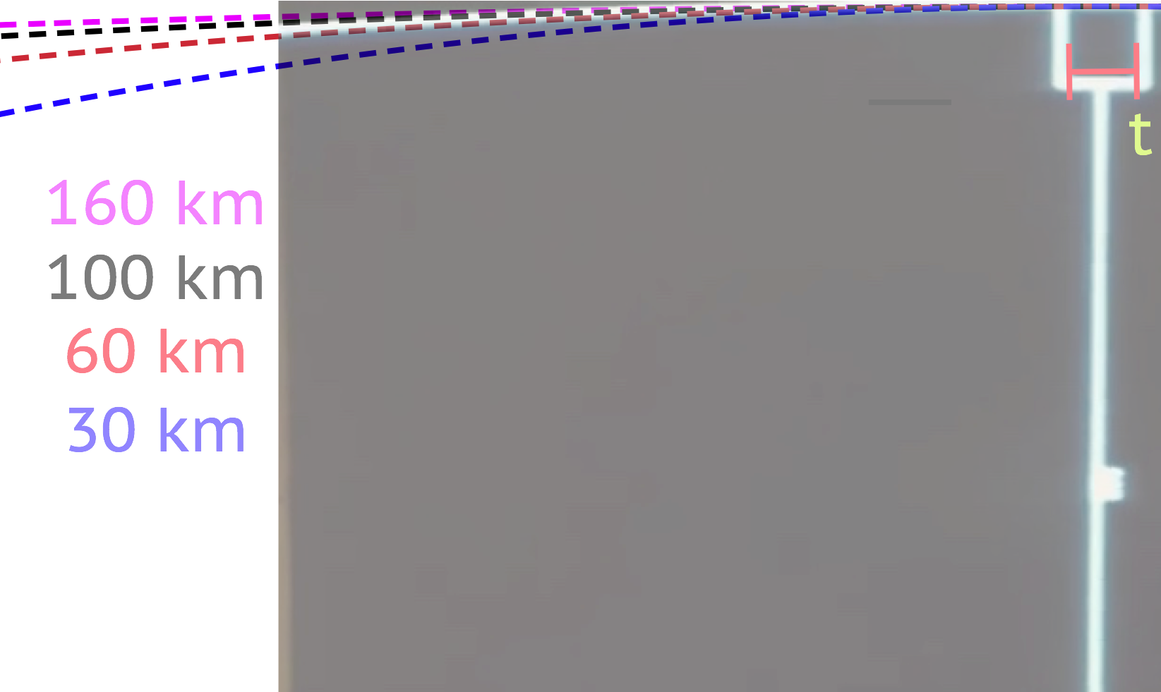
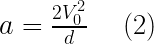
From the previous scale analysis in Part I, the distance from the port, d, and height, h, above the the port can be estimated. They are approximately equal, h = d = 21 meters. The length of the x-wing is L = 12.5 m. After deployment, the trajectory slightly rises and then falls into the exhaust port as shown in Figure 2. A straightforward projectile motion calculation gives the formula for the necessary downward acceleration to follow the trajectory of an object under these conditions

Where t is the launch angle and Vo is the initial horizontal velocity of the projectile. If we assume for simplicity that the angle 
From the surface gravity, the mass of can be obtained, assuming Newtonian gravity,

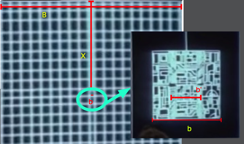
Here G = 1.67E-11 Nm/kg, the gravitational constant. For a bombing run, let’s assume the initial speed of the projectile to be the speed of the x-wing coming down the trench. To estimate the speed, v, of the x-wing, information from the on-board battle computers is used. In Part I, the length of the trench leading to the exhaust port was estimated to be about x = 4.7 kilometers. On the battle computers, the number display coincidentally starts counting down from the range of about 47000 (units not displayed). However, from this connection I will assume that the battle computers are measuring the distance to the launch point in decimeters. From three battle computer approach edits, shown in Clip 1 below, and using the real time length of the different edits, the speed of an x-wing along the trench is estimated to be about 214 meters/second (481 miles/hour). This is close to the cruising speed of a typical airliner — exceptionally fast given the operating conditions, but not unphysical. This gives a realistic 22 seconds for an x-wing to travel down the trench on a bombing run.
Using this speed and the other information, this places the surface gravity of DS1 at about 448 g (where g is the acceleration due to gravity on the surface of the earth). DS1 would have to have a corresponding mass of 2.4E23 kg to be consistent with this.
However, it is clear that considerable liberty was taken in the above analysis and perhaps too much credibility was given to the battle simulation alone, which does not entirely match the dynamics show in the footage of the battle. Upon inspection of the footage, the proton torpedoes are clearly launched with thrust of their own at a speed greater than that of the x-wing. A reasonable estimate might put v (torpedo) to be roughly twice the cruising speed of the x-wing. Moreover, the torpedoes are obviously not launched a mere d = 21 meters from the port (although h = 21 is plausible), rather sufficiently far such that the port is just out of sight in the clip. Finally, the torpedoes enter the port at an awkward angle and appear to be “sucked in.” One might argue that there could be a heat seeking capability in the torpedo. However, this seems unlikely. If this were the case, then it greatly dilutes the narrative of the battle, which strongly indicates not only that the shot was very difficult but that it required the power of the Force to really be successful. Clearly, “heat seeking missiles along with the power of the Force” is a less satisfying message. Indeed, some have speculated that the shot could only have been made by Space Wizards. These scenarios, and other realistic permutations, are in tension with the simulation shown in the briefing. Based on different adjustments of the parameters v (torpedo), h, d, and th, one can tune the value of the surface gravity and mass to be just about anything.
However, if we attempt to be consistent with the battle footage, we might assume again that t=0 degrees while d = 210 m, and v (torpedo) = 2 v (x-wing) for propulsion. The speed of the x-wing can remain the same as before at 214 m/s. Even with this, the surface gravity will be 18g. This still leads to a mass over 10000 times larger than the mass of a realistic superstructure. In this case, a ball of neutronium 18 m in radius could still be contained in the center to account for this mass.
Nevertheless, my analysis is based on the following premise: the simulation indicates that the rebel analysts at least believed, based on the best information available, that a dead drop of a proton torpedo into the port, only under the influence of DS1’s gravity, was at least possible at d = h = 21 meters at the cruising speed of an x-wing flying along the trench under fire nap-of-the-earth. Any dynamics that occurred in real time under battle conditions would ultimately need to be consistent with this.
The large intrinsic surface acceleration may seem problematic (consider tidal forces or other substantial technological complications). However, as demonstrated repeatedly in the Star Wars universe, there already exists exquisite technology to manipulate gravity and create the appropriate artificial gravity conditions to accommodate human activities (e.g. within DS1, the x-wings, etc.) under a very wide range of activities (e.g. acceleration to hyperspace, rapid maneuvering of spacecraft, artificial gravity within spacecraft at arbitrary angles, etc.).
Implications for such a large mass.
One hypothesis that would explain such a large mass would be to assume DS1 had, at its core, a substantial quantity of localized neutrinoium or quark-gluon plasma contained as an energy source. Such a source with high energy density could be used for the purposes of powering a weapon capable of destroying a planet, as an energy source for propulsion, and other support activities. For example, the destiny of neutronium is about 4E17 kilograms per cubic meter and a quark-gluon plasma is about 1E18 kilograms per cubic meter. Specifically, a contained sphere of neutronium at the center of the death star of radius 55 meters would account for the calculated mass and surface gravity of DS1.
It has been estimated that approximately 2.4E32 joules of energy would be required to destroy an earth-sized planet. If 6.7 cubic meters of neutronium (e.g. a sphere of radius 1.88 m) could be converted to useful energy with an efficiency of 0.1%, this would be sufficient to destroy a planet (assuming the supporting technology was in place). This is using the formula
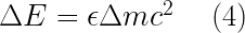
where 


By using the work-energy theorem, the energy required to accelerate DS1 to an arbitrary speed can be estimated. Assuming the possibility for relativistic motion, it can be shown (left as an exerise for the reader) that the volume V of fuel of density 


This does not account for the loss of mass as the fuel is used, so represents an upper limit. For example, to accelerate DS1 with M = 2.4E23 kg from rest to 0.1% the speed of light (0.001 c) would require about 296 cubic meters of neutronium (a sphere of radius 4.1 m).
From this, one concludes that the propulsion system may be the largest energy consideration rather than the primary weapon. For example, consider DS1 enters our solar system from hyperspace (whose energetics are not considered here) and found itself near the orbit of mars. It would take two days for it to travel to earth at 0.001 c.